# Read the data and append SENTENCE_START and SENTENCE_END tokens print"Reading CSV file..." withopen('data/reddit-comments-2015-08.csv', 'rb') as f: reader = csv.reader(f, skipinitialspace=True) reader.next() # Split full comments into sentences sentences = itertools.chain(*[nltk.sent_tokenize(x[0].decode('utf-8').lower()) for x in reader]) # Append SENTENCE_START and SENTENCE_END sentences = ["%s %s %s" % (sentence_start_token, x, sentence_end_token) for x in sentences] print"Parsed %d sentences." % (len(sentences))
# Tokenize the sentences into words tokenized_sentences = [nltk.word_tokenize(sent) for sent in sentences]
# Count the word frequencies word_freq = nltk.FreqDist(itertools.chain(*tokenized_sentences)) print"Found %d unique words tokens." % len(word`_freq.items())
# Get the most common words and build index_to_word and word_to_index vectors vocab = word_freq.most_common(vocabulary_size-1) index_to_word = [x[0] for x in vocab] index_to_word.append(unknown_token) word_to_index = dict([(w,i) for i,w inenumerate(index_to_word)])
print"Using vocabulary size %d." % vocabulary_size print"The least frequent word in our vocabulary is '%s' and appeared %d times." % (vocab[-1][0], vocab[-1][1])
# Replace all words not in our vocabulary with the unknown token for i, sent inenumerate(tokenized_sentences): tokenized_sentences[i] = [w if w in word_to_index else unknown_token for w in sent]
# Create the training data X_train = np.asarray([[word_to_index[w] for w in sent[:-1]] for sent in tokenized_sentences]) y_train = np.asarray([[word_to_index[w] for w in sent[1:]] for sent in tokenized_sentences])
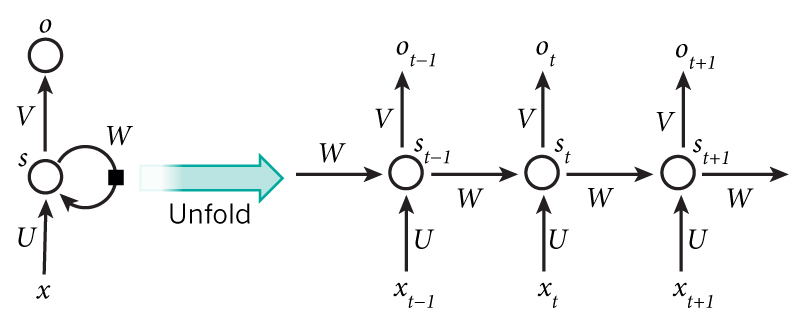
以下是一个训练样本:
1
2
3
4
5
6
7
x:
SENTENCE_START what are n't you understanding about this ? !
[0, 51, 27, 16, 10, 856, 53, 25, 34, 69]

y:
what are n't you understanding about this ? ! SENTENCE_END
[51, 27, 16, 10, 856, 53, 25, 34, 69, 1]
defforward_propagation(self, x): # The total number of time steps T = len(x) # During forward propagation we save all hidden states in s because need them later. # We add one additional element for the initial hidden, which we set to 0 s = np.zeros((T + 1, self.hidden_dim)) s[-1] = np.zeros(self.hidden_dim) # The outputs at each time step. Again, we save them for later. o = np.zeros((T, self.word_dim)) # For each time step... for t in np.arange(T): # Note that we are indxing U by x[t]. This is the same as multiplying U with a one-hot vector. s[t] = np.tanh(self.U[:,x[t]] + self.W.dot(s[t-1])) o[t] = softmax(self.V.dot(s[t])) return [o, s]
defpredict(self, x): # Perform forward propagation and return index of the highest score o, s = self.forward_propagation(x) return np.argmax(o, axis=1)
defcalculate_total_loss(self, x, y): L = 0 # For each sentence... for i in np.arange(len(y)): o, s = self.forward_propagation(x[i]) # We only care about our prediction of the "correct" words correct_word_predictions = o[np.arange(len(y[i])), y[i]] # Add to the loss based on how off we were L += -1 * np.sum(np.log(correct_word_predictions)) return L
defcalculate_loss(self, x, y): # Divide the total loss by the number of training examples N = np.sum((len(y_i) for y_i in y)) return self.calculate_total_loss(x,y)/N
Limit to 1000 examples to save time print"Expected Loss for random predictions: %f" % np.log(vocabulary_size) print"Actual loss: %f" % model.calculate_loss(X_train[:1000], y_train[:1000])
defgradient_check(self, x, y, h=0.001, error_threshold=0.01): # Calculate the gradients using backpropagation. We want to checker if these are correct. bptt_gradients = self.bptt(x, y) # List of all parameters we want to check. model_parameters = ['U', 'V', 'W'] # Gradient check for each parameter for pidx, pname inenumerate(model_parameters): # Get the actual parameter value from the mode, e.g. model.W parameter = operator.attrgetter(pname)(self) print"Performing gradient check for parameter %s with size %d." % (pname, np.prod(parameter.shape)) # Iterate over each element of the parameter matrix, e.g. (0,0), (0,1), ... it = np.nditer(parameter, flags=['multi_index'], op_flags=['readwrite']) whilenot it.finished: ix = it.multi_index # Save the original value so we can reset it later original_value = parameter[ix] # Estimate the gradient using (f(x+h) - f(x-h))/(2*h) parameter[ix] = original_value + h gradplus = self.calculate_total_loss([x],[y]) parameter[ix] = original_value - h gradminus = self.calculate_total_loss([x],[y]) estimated_gradient = (gradplus - gradminus)/(2*h) # Reset parameter to original value parameter[ix] = original_value # The gradient for this parameter calculated using backpropagation backprop_gradient = bptt_gradients[pidx][ix] # calculate The relative error: (|x - y|/(|x| + |y|)) relative_error = np.abs(backprop_gradient - estimated_gradient)/(np.abs(backprop_gradient) + np.abs(estimated_gradient)) # If the error is to large fail the gradient check if relative_error > error_threshold: print"Gradient Check ERROR: parameter=%s ix=%s" % (pname, ix) print"+h Loss: %f" % gradplus print"-h Loss: %f" % gradminus print"Estimated_gradient: %f" % estimated_gradient print"Backpropagation gradient: %f" % backprop_gradient print"Relative Error: %f" % relative_error return it.iternext() print"Gradient check for parameter %s passed." % (pname)
RNNNumpy.gradient_check = gradient_check
# To avoid performing millions of expensive calculations we use a smaller vocabulary size for checking. grad_check_vocab_size = 100 np.random.seed(10) model = RNNNumpy(grad_check_vocab_size, 10, bptt_truncate=1000) model.gradient_check([0,1,2,3], [1,2,3,4])
接下来我们实现SGD。
###实现SGD
通过两步实现:
sdg_step计算计算梯度对每个batch更新
外部循环迭代整个训练数据并且调整学习率
1 2 3 4 5 6 7 8 9
defnumpy_sdg_step(self, x, y, learning_rate): # Calculate the gradients dLdU, dLdV, dLdW = self.bptt(x, y) # Change parameters according to gradients and learning rate self.U -= learning_rate * dLdU self.V -= learning_rate * dLdV self.W -= learning_rate * dLdW
Outer SGD Loop # - model: The RNN model instance # - X_train: The training data set # - y_train: The training data labels # - learning_rate: Initial learning rate for SGD # - nepoch: Number of times to iterate through the complete dataset # - evaluate_loss_after: Evaluate the loss after this many epochs deftrain_with_sgd(model, X_train, y_train, learning_rate=0.005, nepoch=100, evaluate_loss_after=5): # We keep track of the losses so we can plot them later losses = [] num_examples_seen = 0 for epoch inrange(nepoch): # Optionally evaluate the loss if (epoch % evaluate_loss_after == 0): loss = model.calculate_loss(X_train, y_train) losses.append((num_examples_seen, loss)) time = datetime.now().strftime('%Y-%m-%d %H:%M:%S') print"%s: Loss after num_examples_seen=%d epoch=%d: %f" % (time, num_examples_seen, epoch, loss) # Adjust the learning rate if loss increases if (len(losses) > 1and losses[-1][1] > losses[-2][1]): learning_rate = learning_rate * 0.5 print"Setting learning rate to %f" % learning_rate sys.stdout.flush() # For each training example... for i inrange(len(y_train)): # One SGD step model.sgd_step(X_train[i], y_train[i], learning_rate) num_examples_seen += 1
完成。我们来测试一下训练耗费多长的时间:
1 2 3
np.random.seed(10) model = RNNNumpy(vocabulary_size) %timeit model.sgd_step(X_train[10], y_train[10], 0.005)
np.random.seed(10) # Train on a small subset of the data to see what happens model = RNNNumpy(vocabulary_size) losses = train_with_sgd(model, X_train[:100], y_train[:100], nepoch=10, evaluate_loss_after=1)
1 2 3 4 5 6 7 8 9 10
2016-06-1316:59:46: Loss after num_examples_seen=0 epoch=0: 8.987425 2016-06-1316:59:56: Loss after num_examples_seen=100 epoch=1: 8.976270 2016-06-1317:00:06: Loss after num_examples_seen=200 epoch=2: 8.960212 2016-06-1317:00:16: Loss after num_examples_seen=300 epoch=3: 8.930430 2016-06-1317:00:26: Loss after num_examples_seen=400 epoch=4: 8.862264 2016-06-1317:00:37: Loss after num_examples_seen=500 epoch=5: 6.913570 2016-06-1317:00:46: Loss after num_examples_seen=600 epoch=6: 6.302493 2016-06-1317:00:56: Loss after num_examples_seen=700 epoch=7: 6.014995 2016-06-1317:01:06: Loss after num_examples_seen=800 epoch=8: 5.833877 2016-06-1317:01:16: Loss after num_examples_seen=900 epoch=9: 5.710718
看起来,SGD起到了效果。
##通过Theano和GPU训练
1
2
3
enp.random.seed(10) model = RNNTheano(vocabulary_size) %timeit model.sgd_step(X_train[10], y_train[10], 0.005)
这次一次SGD步骤耗费为73.7ms。
这里我们直接使用训练好的的参数:
1 2 3 4 5 6
from utils import load_model_parameters_theano, save_model_parameters_theano
defgenerate_sentence(model): # We start the sentence with the start token new_sentence = [word_to_index[sentence_start_token]] # Repeat until we get an end token whilenot new_sentence[-1] == word_to_index[sentence_end_token]: next_word_probs = model.forward_propagation(new_sentence) sampled_word = word_to_index[unknown_token] # We don't want to sample unknown words while sampled_word == word_to_index[unknown_token]: samples = np.random.multinomial(1, next_word_probs[-1]) sampled_word = np.argmax(samples) new_sentence.append(sampled_word) sentence_str = [index_to_word[x] for x in new_sentence[1:-1]] return sentence_str
num_sentences = 10 senten_min_length = 7
for i inrange(num_sentences): sent = [] # We want long sentences, not sentences with one or two words whilelen(sent) < senten_min_length: sent = generate_sentence(model) print" ".join(sent)